Exporter Tutorial

This tutorial walks through exporting a Reinforcement Learning environment and its policy to a self-contained ONNX file using exploy.exporter.core. Rather than exporting only the neural network, exploy captures the entire environment logic — observation computation, action processing, and any additional inputs and outputs — into a single ONNX graph. This ensures the exported model behaves identically in simulation and on hardware.

By the end of this tutorial you will know how to:

1. Create an exportable adapter for an existing environment.

2. Register inputs, outputs, and memory with the context manager.

3. Create an actor (policy network).

4. Export the environment to ONNX.

5. Load and run the exported model.

6. Validate the export by comparing ONNX outputs against the original environment.

Note: A complete, runnable version of the code in this tutorial is available as a test in python/exploy/exporter/core/tests/test_export_environment.py. This tutorial explains the details behind that test step by step.

Prerequisites

The tutorial uses the following imports:

import pathlib
import tempfile

import torch

from exploy.exporter.core.actor import ExportableActor, add_actor_memory
from exploy.exporter.core.context_manager import Group, Input, Memory, Output
from exploy.exporter.core.evaluator import evaluate, evaluate_episode
from exploy.exporter.core.exportable_environment import ExportableEnvironment
from exploy.exporter.core.exporter import export_environment_as_onnx
from exploy.exporter.core.session_wrapper import SessionWrapper

---

Step 1 — Define the Data Source and the Environment

Before we can export anything, we need an environment to export. In a real project this would typically be a simulation environment (e.g., from IsaacLab or another RL framework). For this tutorial we define a minimal data source and environment from scratch.

Data source

An environment typically reads state from some external source (sensors, a simulator, etc.). Here we create a simple DataSource that holds a few tensors and can step and reset them:

class DataSource:
    """Provides state tensors to the environment."""

    def __init__(self):
        self._init_foo = torch.Tensor([[1.0, 2.0, 3.0, 4.0]])
        self._init_bar = torch.Tensor([[0.5, 0.6]])
        self._init_baz = torch.Tensor([[-7.0, -8.0]])

        self.foo = self._init_foo.clone()
        self.bar = self._init_bar.clone()
        self.baz = self._init_baz.clone()

    def reset(self):
        """Reset to initial state."""
        self.foo[:] = self._init_foo
        self.bar[:] = self._init_bar
        self.baz[:] = self._init_baz

    def step(self):
        """Advance state to emulate a changing environment."""
        self.foo[:] += 0.1
        self.bar[:] += 0.2
        self.baz[:] += 0.3

The data source stores its initial values so it can be reset, and its step() method mutates the tensors in place — just like a physics simulator would update joint positions and velocities each tick.

Environment

The Environment class represents a standard RL environment. It owns a DataSource, computes observations from the state tensors, processes and applies actions, and implements a step() method that advances the simulation:

class Environment:
    """A simple Reinforcement Learning environment."""

    def __init__(self, data_source: DataSource):
        self._data_source = data_source
        self._decimation = 4
        self._actions = torch.zeros(1, 2)
        self._processed_action = torch.zeros_like(self._actions)
        self._output = torch.zeros_like(self._actions)

        self._reset_after_steps = 10
        self._step_count = 0

    @property
    def num_act(self) -> int:
        return self._actions.shape[-1]

    @property
    def num_obs(self) -> int:
        return self.compute_obs().shape[-1]

    @property
    def data_source(self):
        return self._data_source

    def compute_obs(self) -> torch.Tensor:
        return torch.cat(
            [
                self.data_source.foo + 1.0,
                self.data_source.bar + 2.0 * self.data_source.baz,
                self.data_source.baz,
                self._actions,
            ],
            dim=-1,
        )

    def process_actions(self, actions: torch.Tensor):
        self._actions[:] = actions
        self._processed_action[:] = 3 * actions

    def apply_actions(self):
        self._output[:] = self._processed_action + 2

    def step(self, actions: torch.Tensor) -> tuple[torch.Tensor, bool]:
        done = False

        self.process_actions(actions)

        for _ in range(self._decimation):
            self.apply_actions()
            self.data_source.step()

        self._step_count += 1

        if self._step_count >= self._reset_after_steps:
            self._step_count = 0
            self._data_source.reset()
            self._actions[:] = torch.zeros_like(self._actions)
            done = True

        obs = self.compute_obs()
        return obs, done

Note that compute_obs() uses only torch operations — it concatenates tensors from the data source together with the current actions. This is important because these operations will be traced during ONNX export.

At this point, DataSource and Environment are plain Python classes with no dependency on exploy. The next step is to create an adapter that makes the environment exportable.

---

Step 2 — Implement the Exportable Environment Adapter

The exporter needs a standardized interface to trace observation computation, action processing, and simulation stepping. This interface is defined by the ExportableEnvironment abstract base class.

Rather than modifying the original Environment class, create a thin adapter — ExportableEnv — that wraps it and delegates each method:

class ExportableEnv(ExportableEnvironment):
    """Adapter that makes an Environment exportable to ONNX."""

    def __init__(self, env: Environment):
        super().__init__()
        self._env = env

    @property
    def env(self) -> Environment:
        return self._env

    # -- Required abstract methods -------------------------------------------------

    def compute_observations(self) -> torch.Tensor:
        return self.env.compute_obs()

    def process_actions(self, actions: torch.Tensor):
        return self.env.process_actions(actions)

    def apply_actions(self):
        return self.env.apply_actions()

    def step(self, actions: torch.Tensor) -> tuple[torch.Tensor, bool]:
        return self.env.step(actions)

    @property
    def decimation(self) -> int:
        return self.env._decimation

    def prepare_export(self):
        pass

    def empty_actor_observations(self) -> torch.Tensor:
        return torch.zeros_like(self.env.compute_obs())

    def empty_actions(self) -> torch.Tensor:
        return torch.zeros_like(self.env._actions)

    def metadata(self) -> dict:
        return {"env_name": "Env", "version": "1.0"}

    def register_evaluation_hooks(self, update, evaluate_substep):
        pass

    def get_observation_names(self) -> list[str]:
        obs1_names = [f"foo_{i}" for i in range(self.env.data_source.foo.shape[-1])]
        obs2_names = [f"bar_{i}" for i in range(self.env.data_source.bar.shape[-1])]
        obs3_names = [f"baz_{i}" for i in range(self.env.data_source.baz.shape[-1])]
        obs4_names = [f"actions_{i}" for i in range(self.env._actions.shape[-1])]
        return obs1_names + obs2_names + obs3_names + obs4_names

    def observations_reset(self) -> torch.Tensor:
        return self.env.compute_obs()

A few things to note about the methods:

• compute_observations() — Must use only traceable torch operations so the computation graph can be captured during ONNX export. The adapter delegates to env.compute_obs(), which already satisfies this requirement.

• process_actions() / apply_actions() — Split the action pipeline so the exporter can trace the path from raw actions to commanded outputs at the simulation time-step rate.

• decimation — The number of simulation sub-steps per policy step (e.g., policy runs at 50 Hz while simulation runs at 200 Hz → decimation = 4).

• step() — Called during evaluation to advance the environment. Returns updated observations and a flag indicating whether a reset occurred.

• metadata() — Arbitrary key-value pairs that are embedded in the exported ONNX file.

---

Step 3 — Register Inputs, Outputs, and Memory

The exporter traces the torch operations inside compute_observations() to build the ONNX graph, but it also needs to know which tensors correspond to named inputs and outputs of the graph. This is where the context manager comes in.

Looking at compute_obs() from Step 1, the observation is computed from three state tensors (foo, bar, baz) and the previous actions:

torch.cat(
    [
        self.data_source.foo + 1.0,
        self.data_source.bar + 2.0 * self.data_source.baz,
        self.data_source.baz,
        self._actions,
    ],
    dim=-1,
)

Each of these tensors needs to be declared so the exporter knows how to feed data into the ONNX graph at inference time. Additionally, the environment produces an output (self._output) that we want to read back after each inference call. We register all of these on the ContextManager using three component types:

Component	Direction	Purpose
Input	Into the graph	Raw state data read from the robot/simulator
Output	Out of the graph	Computed values to send to the robot/simulator
Memory	Both	Values that persist across inference calls

foo, bar, and baz come from the data source and change every step — these are inputs. The processed action result self._output is something the controller needs to read back — this is an output. The previous actions (self._actions) are used in the observation computation and need to persist from one inference call to the next — this is memory.

Register them on the exportable environment’s context manager:

data_source = DataSource()
env = Environment(data_source=data_source)
exp_env = ExportableEnv(env=env)

exp_env.context_manager().add_components(
    [
        # foo is an input: it feeds into compute_observations() from the data source.
        Input(
            name="foo",
            get_from_env_cb=lambda: exp_env.env.data_source.foo,
            metadata={"description": "The foo tensor from the data source."},
        ),
        # out is an output: it carries the result of apply_actions() back to the caller.
        Output(
            name="out",
            get_from_env_cb=lambda: exp_env.env._output,
            metadata={"description": "The output tensor computed from the actions."},
        ),
        # actions is memory: it is used inside compute_observations() and must persist
        # across inference calls because the observation includes the previous actions.
        Memory(
            name="actions",
            get_from_env_cb=lambda: exp_env.env._actions,
        ),
        # processed_action is memory: it is updated in-place by apply_actions() and must
        # persist across inference calls.
        Memory(
            name="process_actions",
            get_from_env_cb=lambda: exp_env.env._processed_action,
        ),
    ]
)

Each component takes a name and a get_from_env_cb callback that returns the corresponding tensor from the environment. Optionally, you can attach metadata as a dictionary — these key-value pairs are embedded in the exported ONNX file and can be read at deployment time.

Inputs Are Wired by Object Identity

An input only becomes an ONNX graph input if the exact tensor object returned by its callback is read during the traced compute_observations() call. Callbacks that return a stored tensor (like foo, bar, and baz above) satisfy this naturally. A callback that computes a fresh tensor does not: the observation computation produces a different object during tracing, so the registered input dangles and is silently dropped from the exported graph — the exporter prints an informational message listing such inputs after export.

To use a derived quantity (an arbitrary function of the environment state) as a graph input, it must be materialized as a stored tensor first. Declare the quantity once as a DerivedTensor (compute function and optional split dimension), call materialize(data) with the data-source proxy when registering inputs, and call the object itself wherever the value is needed — it returns the stored leaf during export and falls back to computing the quantity live once the proxy is discarded (during training or post-export evaluation). See Advanced: Derived Input Tensors for a worked example (body velocities expressed in each body’s own frame).

Grouping Related Inputs

Related inputs can be organized into a Group. This is purely organizational and does not affect the export — it simply lets you add multiple inputs together with shared metadata:

exp_env.context_manager().add_group(
    Group(
        name="bar_baz_group",
        items=[
            Input(
                name="bar",
                get_from_env_cb=lambda: exp_env.env.data_source.bar,
            ),
            Input(
                name="baz",
                get_from_env_cb=lambda: exp_env.env.data_source.baz,
            ),
        ],
        metadata={"description": "A group of related inputs."},
    )
)

---

Step 4 — Create an Actor

The actor is the policy network. Subclass ExportableActor and implement forward():

class Actor(ExportableActor):
    """A simple MLP policy network."""

    def __init__(self, num_obs: int, num_act: int):
        super().__init__()

        self._net = torch.nn.Sequential(
            torch.nn.Linear(num_obs, 10),
            torch.nn.ELU(),
            torch.nn.Linear(10, 10),
            torch.nn.ReLU(),
            torch.nn.Linear(10, num_act),
            torch.nn.ELU(),
        )

    def forward(self, x: torch.Tensor) -> torch.Tensor:
        return self._net(x)

Create the actor in evaluation mode:

actor = Actor(num_obs=env.num_obs, num_act=env.num_act).eval()

Calling .eval() is important — it disables dropout and batch-norm training behavior, ensuring deterministic inference during export and evaluation.

---

Step 5 — Export to ONNX

With the exportable environment, context manager, and actor ready, export everything to a single ONNX file using export_environment_as_onnx():

export_path = pathlib.Path("/tmp/exploy_tutorial")
onnx_file_name = "policy.onnx"

export_environment_as_onnx(
    env=exp_env,
    actor=actor,
    path=export_path,
    filename=onnx_file_name,
    verbose=False,
)

This traces all registered torch operations — observation computation, the actor network, action processing — and writes them into a single ONNX graph. The resulting file contains the full computation pipeline from raw inputs to commanded outputs, along with the metadata you registered.

Inspecting and understanding the generated ONNX files

When exporting an environment and its actor, Exploy produces policy.onnx (or whatever filename is passed to export_environment_as_onnx()). That exported file can then be used for evaluation (see Putting It All Together) or for deployment in a controller (see Controller Tutorial).

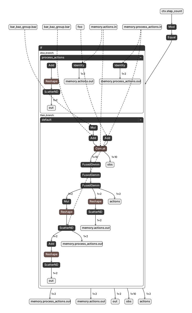
The export contains two execution paths by design: Default and ProcessActions. The Default path runs at the policy rate and includes observation computation plus actor inference, while the ProcessActions path runs at the simulation rate and captures the computational graph for action post-processing and command application that occurs at every simulation sub-step. This separation preserves the original control timing (policy step vs. simulation sub-step) in the exported model.

Additionally, Exploy will produce debug computational graphs. These are only to be used for debugging and visual inspection.

• debug/policy_default.onnx: The Default path of the computational graph.

• debug/policy_process_actions.onnx: The ProcessActions path of the computational graph.

• debug/policy_optimized.onnx: The optimized version of the exported ONNX model.

Note: debug/policy_optimized.onnx is generated when optimize=True is passed to SessionWrapper. While fully functional, it requires the same ONNX Runtime version to be used in both the exporter and the controller. This constraint depends on the user’s setup. For deployment in a controller, only the policy.onnx file should be used.

Visualizing the Exported ONNX Graph

You can inspect the exported ONNX file using Netron, an open-source viewer for neural network models. The screenshots below show the computational graphs produced by the export steps in this tutorial. The unit test runs on three different environments:

• an environment that computes observations and uses an MLP actor

• an environment that uses a torch module to compute parts of its observations and uses an MLP actor

• an environment that uses a torch module to compute parts of its observations and uses an RNN-based actor

Each exported ONNX file contains two subgraphs: a Default graph that computes observations and actions at the policy rate, and a ProcessActions graph that maps raw actions to commanded outputs at the simulation rate.

Environment and MLP Actor

This is the full default graph for the basic Environment from Step 1. You can see the named inputs (foo), the group inputs (bar, baz), and the memory inputs (memory.actions.in) flowing through the observation computation and into the actor network, which produces actions and the named outputs (out, memory.actions.out). The ProcessActions subgraph traces only process_actions() and apply_actions(). It runs at the simulation time-step rate (i.e., once per decimation sub-step) and maps actions to commanded outputs.

Environment with a torch module and MLP Actor

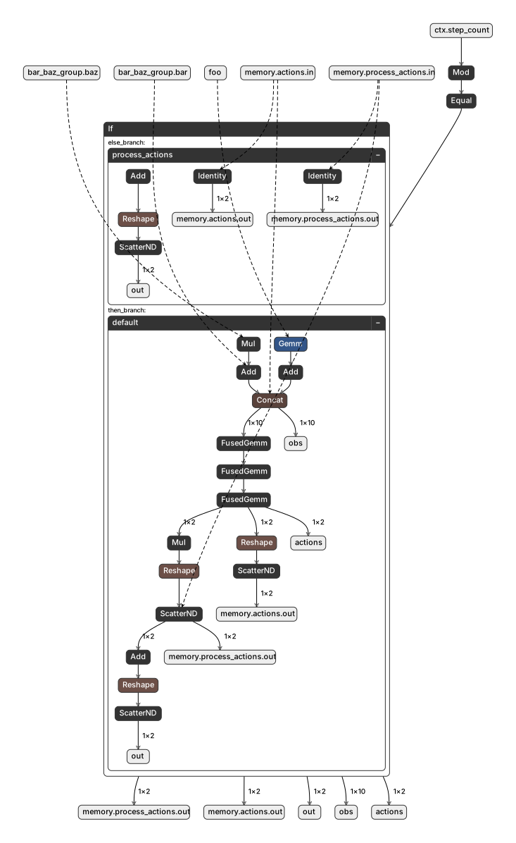
When the environment includes a learnable torch.nn.Module (see the Advanced: Using Torch Modules in Observations section), the module’s parameters and operations appear in the graph:

Environment with a torch module and an RNN Actor

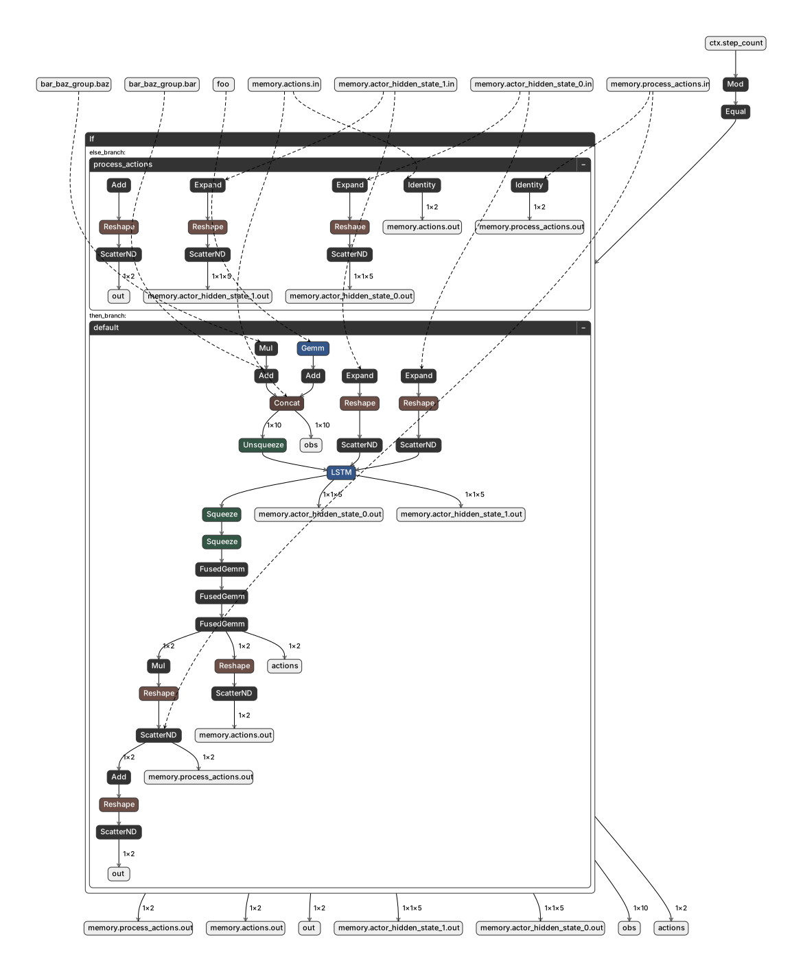
When using an RNN-based actor (see Advanced: RNN-Based Actors), the graph includes the LSTM hidden states as additional memory inputs and outputs:

---

Step 6 — Load and Run the Exported Model

Use SessionWrapper to load the ONNX file and run inference:

session_wrapper = SessionWrapper(
    onnx_folder=export_path,
    onnx_file_name=onnx_file_name,
    actor=actor,
    optimize=True,
)

Setting optimize=True enables ONNX Runtime graph optimizations for faster inference. The actor parameter is optional — it is stored for use during evaluation, but inference runs entirely through the ONNX graph.

---

Step 7 — Evaluate the Export

The evaluate() function runs the environment and the ONNX session side by side, comparing their outputs at every step:

with torch.inference_mode():
    export_ok, observations = evaluate(
        env=exp_env,
        context_manager=exp_env.context_manager(),
        session_wrapper=session_wrapper,
        num_episodes=1,
        max_episode_steps=20,
        verbose=True,
        pause_on_failure=False,
    )

evaluate() returns:

• export_ok (bool) — True if all outputs matched within tolerance across all steps.

• observations (torch.Tensor) — The final observations after evaluation.

If export_ok is False, the evaluator prints a detailed diagnostic showing which outputs diverged and at which step.

Under the hood, evaluate() calls evaluate_episode() once per episode. You can call evaluate_episode() directly when you want finer control — for example, to run and inspect a single episode in a tight debugging loop without the outer episode iteration:

with torch.inference_mode():
    episode_ok, observations = evaluate_episode(
        env=exp_env,
        context_manager=exp_env.context_manager(),
        session_wrapper=session_wrapper,
        max_num_steps=20,
        verbose=True,
        pause_on_failure=False,
    )

---

Advanced: Using Torch Modules in Observations

If your observation computation includes learnable torch modules (e.g., a normalization layer or a learned feature extractor), you need to register them so the exporter includes their parameters in the ONNX graph.

Create an environment that uses a torch.nn.Module inside compute_obs():

class EnvironmentWithTorchModule(Environment):
    """An environment that uses a torch Module in observation computation."""

    def __init__(self, data_source: DataSource):
        module_dim_in = data_source.foo.shape[-1]
        module_dim_out = module_dim_in
        self._module = torch.nn.Linear(module_dim_in, module_dim_out)
        super().__init__(data_source=data_source)

    @property
    def module(self) -> torch.nn.Module:
        return self._module

    def compute_obs(self) -> torch.Tensor:
        return torch.cat(
            [
                self._module(self.data_source.foo) + 1.0,
                self.data_source.bar + 2.0 * self.data_source.baz,
                self.data_source.baz,
                self._actions,
            ],
            dim=-1,
        )

The ExportableEnv adapter from Step 2 works with this subclass without modification, since it delegates to env.compute_obs(). The key additional step is registering the module with the context manager before exporting:

data_source = DataSource()
env = EnvironmentWithTorchModule(data_source=data_source)
exp_env = ExportableEnv(env=env)
actor = Actor(num_obs=env.num_obs, num_act=env.num_act).eval()

# Register the module so its parameters are included in the ONNX graph.
exp_env.context_manager().add_module(env.module)

After this, the standard export and evaluation workflow works unchanged — the module’s learned weights will be embedded in the ONNX file.

---

Advanced: RNN-Based Actors

For policies that use recurrent networks (e.g., LSTM), the hidden state must persist across inference calls. Subclass ExportableActor and implement reset() and get_state():

class RNNActor(ExportableActor):
    """An LSTM-based policy network with persistent hidden state."""

    def __init__(self, num_obs: int, num_act: int):
        super().__init__()

        hidden_dim = 5
        num_rnn_layers = 1

        self._rnn = torch.nn.LSTM(
            input_size=num_obs,
            hidden_size=hidden_dim,
            num_layers=num_rnn_layers,
            batch_first=False,
        )

        self._net = Actor(num_obs=hidden_dim, num_act=num_act)
        self._state = None

    def reset(self, dones: torch.Tensor):
        if self._state is None:
            return
        for state in self._state:
            state[:, dones, :] = 0.0

    def forward(self, x: torch.Tensor) -> torch.Tensor:
        rnn_out, self._state = self._rnn(x.unsqueeze(dim=0), self._state)
        return self._net(rnn_out.squeeze(dim=0))

    def get_state(self) -> tuple[torch.Tensor, ...] | None:
        return self._state

Two additional steps are required when exporting an RNN actor:

1. Initialize the hidden state by running a forward pass before export.

2. Register the hidden state as memory using add_actor_memory().

data_source = DataSource()
env = EnvironmentWithTorchModule(data_source=data_source)
exp_env = ExportableEnv(env=env)
exp_env.context_manager().add_module(env.module)

actor = RNNActor(num_obs=env.num_obs, num_act=env.num_act).eval()

# Initialize the hidden state.
actor(exp_env.empty_actor_observations())

# Register hidden states as memory in the context manager.
add_actor_memory(
    context_manager=exp_env.context_manager(),
    get_hidden_states_func=actor.get_state,
)

add_actor_memory() reads the hidden state tensors from the actor and registers each one as a Memory component. This ensures the ONNX graph exposes them as both inputs and outputs, so the inference runtime can feed the previous hidden state back in at each step.

After this setup, export and evaluate as usual.

---

Advanced: Derived Input Tensors

Some quantities you want to feed the policy are not stored directly on the simulator’s data source — they are derived from other state. A common example is a body’s linear and angular velocity expressed in that body’s own frame: many simulators only expose per-body velocities in the world frame, so the body-frame quantities must be computed by rotating the world-frame velocities by the inverse of the body orientation.

As explained in Inputs Are Wired by Object Identity, a callback that computes a fresh tensor cannot become a graph input: the observation computation produces a different object during tracing, so the registered input dangles and is dropped. To turn a derived quantity into a graph boundary it must first be materialized as a stored leaf tensor. The stored value is registered against the data-source proxy it was computed from, so its lifetime follows the export data-source swap.

Declaring a derived tensor

Declare the quantity once as a DerivedTensor, bundling a compute function and an optional split dimension. The compute function can be any callable with any signature — a free function, a bound method, or a callable class instance — since materialize(...) and calls of the DerivedTensor forward their *args and **kwargs to it unchanged, and materialized values are keyed by the identity of all call arguments. Splitting wraps the stored value in a TensorProxy so that each slice along that dimension (e.g. each body) is an independent leaf — one ONNX input per body:

import torch

import isaaclab.utils.math as math_utils

from exploy.exporter.core.derived_tensors import DerivedTensor
from exploy.exporter.core.tensor_proxy import to_tensor


def _compute_body_link_lin_vel_b(data) -> torch.Tensor:
    return math_utils.quat_apply_inverse(
        to_tensor(data.body_link_quat_w), to_tensor(data.body_link_lin_vel_w)
    )


def _compute_body_link_ang_vel_b(data) -> torch.Tensor:
    return math_utils.quat_apply_inverse(
        to_tensor(data.body_link_quat_w), to_tensor(data.body_link_ang_vel_w)
    )


# Body link velocities rt the world frame, expressed in each body's own frame, with shape
# (num_instances, num_bodies, 3). Split along dim 1 so each body becomes its own ONNX input.
body_link_lin_vel_b = DerivedTensor(compute_fn=_compute_body_link_lin_vel_b, split_dim=1)
body_link_ang_vel_b = DerivedTensor(compute_fn=_compute_body_link_ang_vel_b, split_dim=1)

Materializing and registering inputs

Call materialize(data) with the data-source proxy to compute the quantity once and store it as a leaf, then bind each Input to a slice of the stored value. Only materialize the export proxy — its state is a frozen snapshot, whereas materializing live framework data would freeze the quantity while the simulation keeps changing. The framework-shipped derived tensors are materialized automatically when the exportable environment swaps the data sources in; a custom quantity is materialized in the export script, which runs after the swap. Materialize before registering the Inputs: an Input captures the tensor returned by its callback at construction time, and only the stored leaf can become a graph input:

articulation_name = "robot"  # the articulation's name in the scene
data = entity.data  # the ArticulationDataSource / EntityDataSource proxy
body_link_lin_vel_b.materialize(data)
body_link_ang_vel_b.materialize(data)

for idx, body_name in enumerate(entity.body_names):
    context_manager.add_component(
        Input(
            name=f"obj.{articulation_name}.{body_name}.lin_vel_b_rt_w_in_b",
            get_from_env_cb=lambda _entity=entity, i=idx: body_link_lin_vel_b(_entity.data)[:, i],
        )
    )

Because the Input callback returns a slice of the stored leaf, the exact same object is read during tracing and the input becomes a graph boundary supplied by the deployment side.

Reading a derived tensor in an observation term

The same DerivedTensor object is callable and works as a framework observation term in both training and export. During export the leaf has been materialized against the proxy, so tracing reads the stored object; during training (or post-export evaluation, once the original data is restored) the value is computed live:

import torch
from isaaclab.assets import Articulation
from isaaclab.managers import SceneEntityCfg

from exploy.exporter.frameworks.isaaclab.derived_tensors import (
    body_link_ang_vel_b,
    body_link_lin_vel_b,
)


def body_lin_vel_b(env, asset_cfg=SceneEntityCfg("robot")) -> torch.Tensor:
    """Linear velocities of the selected bodies rt the world frame, in each body's own frame."""
    asset: Articulation = env.scene[asset_cfg.name]
    return body_link_lin_vel_b(asset.data)[:, asset_cfg.body_ids].reshape(env.num_envs, -1)


def body_ang_vel_b(env, asset_cfg=SceneEntityCfg("robot")) -> torch.Tensor:
    """Angular velocities of the selected bodies rt the world frame, in each body's own frame."""
    asset: Articulation = env.scene[asset_cfg.name]
    return body_link_ang_vel_b(asset.data)[:, asset_cfg.body_ids].reshape(env.num_envs, -1)

Observation terms do not have to be free functions. Isaac Lab also supports class-based terms — subclasses of ManagerTermBase that are constructed with the term config and the environment, and called like functions afterwards. A DerivedTensor works the same way there, since it is simply called with the asset’s data object:

import torch
from isaaclab.assets import Articulation
from isaaclab.envs import ManagerBasedEnv
from isaaclab.managers import ManagerTermBase, ObservationTermCfg, SceneEntityCfg

from exploy.exporter.frameworks.isaaclab.derived_tensors import body_link_lin_vel_b


class body_lin_vel_b(ManagerTermBase):
    """Linear velocities of the selected bodies rt the world frame, in each body's own frame."""

    def __init__(self, cfg: ObservationTermCfg, env: ManagerBasedEnv):
        super().__init__(cfg, env)
        asset_cfg: SceneEntityCfg = cfg.params["asset_cfg"]
        self._asset: Articulation = env.scene[asset_cfg.name]

    def __call__(self, env: ManagerBasedEnv, asset_cfg: SceneEntityCfg) -> torch.Tensor:
        return body_link_lin_vel_b(self._asset.data)[:, asset_cfg.body_ids].reshape(
            env.num_envs, -1
        )

The same mechanism also works in the other direction: because materialize(...) and calls of a DerivedTensor forward *args and **kwargs to the compute function, the compute function itself can be a callable class instance (e.g. one constructed with the environment) or take additional arguments — the materialized value is keyed by the identity of all call arguments.

Bundling the compute function and split dimension in a single DerivedTensor guarantees that materialization (during export) and live computation (during training) can never use mismatched functions.

Replacing the output of a pretrained encoder

Derived tensors are not limited to kinematic quantities — they cut the ONNX graph at any computed value. A common use case is a pretrained, frozen encoder (e.g. a perception backbone) whose output feeds the policy. Advanced: Using Torch Modules in Observations shows how to embed such a module in the graph with add_module(). If instead the encoder should run outside the exported policy — for example in a separate perception process on the robot — materialize its output as a derived tensor: the latent becomes an ONNX graph input supplied by the deployment side, and the encoder’s weights are not embedded in the exported file.

from exploy.exporter.core.derived_tensors import DerivedTensor

encoder = load_pretrained_encoder().eval()  # frozen, not registered via add_module()

encoder_latent = DerivedTensor(compute_fn=lambda data: encoder(data.camera_features))

The observation computation reads the quantity through the DerivedTensor:

def compute_obs(self) -> torch.Tensor:
    return torch.cat(
        [
            encoder_latent(self.data_source),
            ...,
        ],
        dim=-1,
    )

In the export script, materialize the latent against the export data-source proxy (after the exportable environment has swapped it in, before registering the inputs) and bind an Input to it:

encoder_latent.materialize(data)

context_manager.add_component(
    Input(
        name="encoder.latent",
        get_from_env_cb=lambda: encoder_latent(data),
    )
)

During tracing, compute_obs() reads the stored leaf, so the graph is cut at the latent: encoder.latent becomes a graph input, the encoder is not traced, and any inputs consumed only by the encoder (e.g. the raw camera features) are dropped from the graph. During post-export evaluation, once the original data source is restored and the proxy is discarded, both the observation computation and the input callback fall back to running the encoder live.

---

Putting It All Together

Here is a complete helper function that ties all the steps together — registering components, exporting to ONNX, loading the model, and validating the export:

def export_and_evaluate(
    exp_env: ExportableEnv,
    actor: ExportableActor,
    onnx_file_name: str,
    num_eval_episodes: int,
    max_eval_steps_per_episode: int,
) -> bool:
    # Register inputs, outputs, and memory.
    exp_env.context_manager().add_components(
        [
            Input(
                name="foo",
                get_from_env_cb=lambda: exp_env.env.data_source.foo,
                metadata={"description": "The foo tensor from the data source."},
            ),
            Output(
                name="out",
                get_from_env_cb=lambda: exp_env.env._output,
                metadata={"description": "The output tensor computed from the actions."},
            ),
            Memory(
                name="actions",
                get_from_env_cb=lambda: exp_env.env._actions,
            ),
            Memory(
                name="process_actions",
                get_from_env_cb=lambda: exp_env.env._processed_action,
            ),
        ]
    )

    exp_env.context_manager().add_group(
        Group(
            name="bar_baz_group",
            items=[
                Input(
                    name="bar",
                    get_from_env_cb=lambda: exp_env.env.data_source.bar,
                ),
                Input(
                    name="baz",
                    get_from_env_cb=lambda: exp_env.env.data_source.baz,
                ),
            ],
            metadata={"description": "A group of related inputs."},
        )
    )

    # Export to ONNX.
    with tempfile.TemporaryDirectory() as tmpdir:
        onnx_path = pathlib.Path(tmpdir) / "exploy"

        export_environment_as_onnx(
            env=exp_env,
            actor=actor,
            path=onnx_path,
            filename=onnx_file_name,
            verbose=False,
        )

        # Load the exported model.
        session_wrapper = SessionWrapper(
            onnx_folder=onnx_path,
            onnx_file_name=onnx_file_name,
            actor=actor,
            optimize=True,
        )

        # Evaluate.
        with torch.inference_mode():
            export_ok, _ = evaluate(
                env=exp_env,
                context_manager=exp_env.context_manager(),
                session_wrapper=session_wrapper,
                num_episodes=num_eval_episodes,
                max_episode_steps=max_eval_steps_per_episode,
                verbose=False,
                pause_on_failure=False,
            )

    return export_ok

Basic environment

data_source = DataSource()
env = Environment(data_source=data_source)
exp_env = ExportableEnv(env=env)
actor = Actor(num_obs=env.num_obs, num_act=env.num_act).eval()

assert export_and_evaluate(
    exp_env, actor, "policy.onnx", num_eval_episodes=1, max_eval_steps_per_episode=20
)

Environment with a torch module

data_source = DataSource()
env = EnvironmentWithTorchModule(data_source=data_source)
exp_env = ExportableEnv(env=env)
actor = Actor(num_obs=env.num_obs, num_act=env.num_act).eval()
exp_env.context_manager().add_module(env.module)

assert export_and_evaluate(
    exp_env, actor, "policy_with_module.onnx", num_eval_episodes=1, max_eval_steps_per_episode=20
)

Environment with a torch module and an RNN actor

data_source = DataSource()
env = EnvironmentWithTorchModule(data_source=data_source)
exp_env = ExportableEnv(env=env)
exp_env.context_manager().add_module(env.module)

actor = RNNActor(num_obs=env.num_obs, num_act=env.num_act).eval()
actor(exp_env.empty_actor_observations())
add_actor_memory(
    context_manager=exp_env.context_manager(),
    get_hidden_states_func=actor.get_state,
)

assert export_and_evaluate(
    exp_env, actor, "policy_with_rnn.onnx", num_eval_episodes=1, max_eval_steps_per_episode=20
)